Hinss2021 classification example

This example shows how to use the Hinss2021 dataset with the resting state paradigm.

In this example, we aim to determine the most effective channel selection strategy for the moabb.datasets.Hinss2021 dataset. The pipelines under consideration are:

• Xdawn

• Electrode selection based on time epochs data

• Electrode selection based on covariance matrices

# License: BSD (3-clause)

import warnings

import numpy as np
import seaborn as sns
from matplotlib import pyplot as plt
from pyriemann.channelselection import ElectrodeSelection
from pyriemann.estimation import Covariances
from pyriemann.spatialfilters import Xdawn
from pyriemann.tangentspace import TangentSpace
from sklearn.base import TransformerMixin
from sklearn.discriminant_analysis import LinearDiscriminantAnalysis as LDA
from sklearn.pipeline import make_pipeline

from moabb import set_log_level
from moabb.datasets import Hinss2021
from moabb.evaluations import CrossSessionEvaluation
from moabb.paradigms import RestingStateToP300Adapter


# Suppressing future and runtime warnings for cleaner output
warnings.simplefilter(action="ignore", category=FutureWarning)
warnings.simplefilter(action="ignore", category=RuntimeWarning)

set_log_level("info")

Create util transformer

Let’s create a scikit transformer mixin, that will select electrodes based on the covariance information

class EpochSelectChannel(TransformerMixin):
    """Select channels based on covariance information."""

    def __init__(self, n_chan, cov_est):
        self._chs_idx = None
        self.n_chan = n_chan
        self.cov_est = cov_est

    def fit(self, X, _y=None):
        # Get the covariances of the channels for each epoch.
        covs = Covariances(estimator=self.cov_est).fit_transform(X)
        # Get the average covariance between the channels
        m = np.mean(covs, axis=0)
        # Select the `n_chan` channels having the maximum covariances.
        indices = np.unravel_index(
            np.argpartition(m, -self.n_chan, axis=None)[-self.n_chan :], m.shape
        )
        # We will keep only these channels for the transform step.
        self._chs_idx = np.unique(indices)
        return self

    def transform(self, X):
        return X[:, self._chs_idx, :]

Initialization Process

1. Define the experimental paradigm object (RestingState)

2. Load the datasets

3. Select a subset of subjects and specific events for analysis

# Here we define the mne events for the RestingState paradigm.
events = dict(easy=2, diff=3)
# The paradigm is adapted to the P300 paradigm.
paradigm = RestingStateToP300Adapter(events=events, tmin=0, tmax=0.5)
# We define a list with the dataset to use
datasets = [Hinss2021()]

# To reduce the computation time in the example, we will only use the
# first two subjects.
n__subjects = 2
title = "Datasets: "
for dataset in datasets:
    title = title + " " + dataset.code
    dataset.subject_list = dataset.subject_list[:n__subjects]

Create Pipelines

Pipelines must be a dict of scikit-learning pipeline transformer.

pipelines = {}

pipelines["Xdawn+Cov+TS+LDA"] = make_pipeline(
    Xdawn(nfilter=4), Covariances(estimator="lwf"), TangentSpace(), LDA()
)

pipelines["Cov+ElSel+TS+LDA"] = make_pipeline(
    Covariances(estimator="lwf"), ElectrodeSelection(nelec=8), TangentSpace(), LDA()
)

# Pay attention here that the channel selection took place before computing the covariances:
# It is done on time epochs.
pipelines["ElSel+Cov+TS+LDA"] = make_pipeline(
    EpochSelectChannel(n_chan=8, cov_est="lwf"),
    Covariances(estimator="lwf"),
    TangentSpace(),
    LDA(),
)

Run evaluation

Compare the pipeline using a cross session evaluation.

# Here should be cross-session
evaluation = CrossSessionEvaluation(
    paradigm=paradigm,
    datasets=datasets,
    overwrite=False,
)

results = evaluation.process(pipelines)

2025-02-19 12:22:05,152 INFO MainThread moabb.evaluations.base Processing dataset: Hinss2021

Hinss2021-CrossSession:   0%|          | 0/2 [00:00<?, ?it/s]Subject 1 already processed

Hinss2021-CrossSession:   0%|          | 0/2 [00:00<?, ?it/s]

Here, with the ElSel+Cov+TS+LDA pipeline, we reduce the computation time in approximately 8 times to the Cov+ElSel+TS+LDA pipeline.

print("Averaging the session performance:")
print(results.groupby("pipeline").mean("score")[["score", "time"]])

Averaging the session performance:
                     score      time
pipeline
Cov+ElSel+TS+LDA  0.770303  1.782743
ElSel+Cov+TS+LDA  0.775472  0.366166
Xdawn+Cov+TS+LDA  0.658810  0.322670

Plot Results

Here, we plot the results to compare two pipelines

fig, ax = plt.subplots(facecolor="white", figsize=[8, 4])

sns.stripplot(
    data=results,
    y="score",
    x="pipeline",
    ax=ax,
    jitter=True,
    alpha=0.5,
    zorder=1,
    palette="Set1",
)
sns.pointplot(data=results, y="score", x="pipeline", ax=ax, palette="Set1").set(
    title=title
)

ax.set_ylabel("ROC AUC")
ax.set_ylim(0.3, 1)

plt.show()

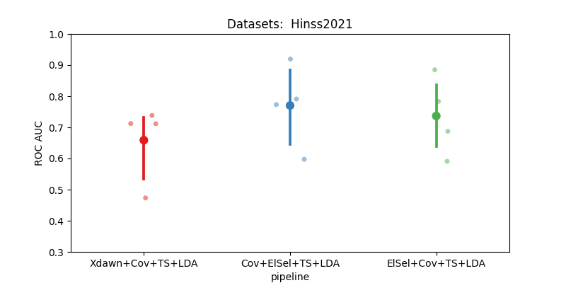
Key Observations:

• Xdawn is not ideal for the resting state paradigm. This is due to its specific design for Event-Related Potential (ERP).

• Electrode selection strategy based on covariance matrices demonstrates less variability and typically yields better performance.

• However, this strategy is more time-consuming compared to the simpler electrode selection based on time epoch data.

Estimated memory usage: 23 MB